Cumulative Model with PSO as an optimizer
Objective
In this project, we developed a process to optimize the allocation of the remaining budget to the platforms for the upcoming quarter by maximizing the predicted conversions through historical spending and conversion data of platform campaigns
Workflow
- Our code extracts weekly conversions of paid UTM campaigns through our multi-touch attribution model (Markov chain) and aggregates them at the platform campaign level. Here, the weekly dates follow the client’s weekly calendar, and the code excludes UTM campaigns that are not mapped to any platform campaign.
- After this, our code extracts every platform campaign’s historical daily spend data and aggregates them at the weekly level. The code is pickling weekly dates according to the client’s calendar.
- The code will merge the above two datasets for delivering historical weekly conversions and the weekly spend of every platform campaign.
- Afterwards, our code defines a new column named ‘program key,’ which combines the name of the platform campaign and platform key to yield a distinct column so that we don’t have to bother when there’s the same name for two platform campaigns on two different platforms.
- To solve the problem of the inactive campaign, our code filters the dataset to consider data for those campaigns that have some spending associated with them in the past 30 days.
- The algorithm filters the campaigns with no cost and no conversions and has less than four records in the past. Because while finding the correlation through linear regression between cumulative spending and cumulative conversions, less than four records will deliver erroneous results.
- Our code then sorts the data of every campaign by its starting week date and calculates two new columns called ‘cumulative spend’ and ‘cumulative conversions.’ As the name suggests, every weekly record of platform campaign will have the sum of all previous spending and current spend. This holds true for conversions as well.
- Then, the code calculates the spend coefficient and R- square value for every platform campaign through linear regression. If we have not put the condition of at least four records of platform campaigns in historical data, then we would have got infinity or 0 as an R – Square value. The linear regression here tries to fit a line between cumulative spend and cumulative conversions, and the slope of that line denotes the spend coefficient.
- After this, we calculate the minimum, and maximum predicted spend for every platform campaign to cap the allocation of every platform campaign.
The minimum capping works like this:
We first calculate the historical spending percentage of every campaign through our filtered dataset. (Remember, it’s not palatable to use the initial, unfiltered dataset because it will include the platform campaigns which are not part of our calculation)
- If the spending percentage is > 10% of the historical filtered dataset, then the minimum spending would be 10% of the remaining budget.
- If the spending percentage is > 1% and <= 10% of the historical filtered dataset, then the minimum spending would be 1% of the remaining budget.
- If the spending percentage is <=1% of the historical filtered dataset, then the minimum spending would be 0.1% of the remaining budget.
The maximum capping works like this:
- If the spending percentage is >= 100% of the historical filtered dataset, then the maximum spending would be 100% of the remaining budget.
- If the spending percentage is >= 80% and < 100% of the historical filtered dataset, the maximum spending would be percent spend of that platform campaign(x%) + 5% of the remaining budget.
- If the spending percentage is >= 50% and < 80% of the historical filtered dataset, the maximum spending would be percent spend of that platform campaign(x%) + 10% of the remaining budget.
- If the spending percentage is >= 30% and < 50% of the historical filtered dataset, the maximum spending would be percent spend of that platform campaign(x%) + 15% of the remaining budget.
- If the spending percentage is >= 10% and < 30% of the historical filtered dataset, the maximum spending would be percent spend of that platform campaign(x%) + 20% of the remaining budget.
- If the spending percentage is >1% and < 10% of the historical filtered dataset, the maximum spending would be percent spend of that platform campaign(x%) + 5% of the remaining budget.
- If the spending percentage is <= 1% of the historical filtered dataset, the maximum spending would be percent spend of that platform campaign(x%) + 1% of the remaining budget.
- For predicting the future spending of every campaign, we won’t be crossing the capping values. So, for predicting and optimizing every campaign spend, we have used Particle Swarm Optimization (PSO). For reading about PSO, you can refer following links:
- https://towardsdatascience.com/particle-swarm-optimization-visually-explained-46289eeb2e14
- https://analyticsindiamag.com/a-tutorial-on-particle-swarm-optimization-in-python/
- https://nathanrooy.github.io/posts/2016-08-17/simple-particle-swarm-optimization-with-python/
- https://machinelearningmastery.com/a-gentle-introduction-to-particle-swarm-optimization/
Note: To fathom the points given below, the reader should have a basic understanding of PSO.
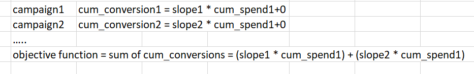
- We have used a modified PSO algorithm in which we are trying to maximize the objective function instead of minimizing it. Here the output function of our optimization function will represent the cumulative conversions for the upcoming quarter. We will be endeavouring to maximize the sum of (spending coefficient * allocated dollars) of every platform campaign. The next version will be applying diminishing effect on allocated dollars.
Diminishing effect
- We changed the signs of velocity and position update in our modified PSO. While looking for the group and individual best, our PSO always tries to find the maximum output of the objective function, which is our need. We have also adjusted the input variable for PSO to undertake any number of campaigns fed to it.
- In PSO, we include the capping conditions. If any platform campaign goes beyond its capping value, our code is smart enough to bring down that value. This holds true for minimum capping as well.
- After trying a variety of values of inertia weight(w), cognitive constant(c1), and social constant(c2), we concluded that our model works satisfactory for w = 0.7, c1 = c2 = 1.496, which are values mentioned in many research papers founded empirically and gratifying many convergence conditions. We also used linear inertia weight, but it’s not working well with our model.
- In our model, we define a list of the number of particles (a hyperparameter in PSO) which helps us to exhaust as well as optimize the remaining budget. It was founded by us empirically while testing and needs more attention. After all this, we observed one more thing, every time we ran PSO, it gave different results, and that was due to the nature of PSO, in which sometimes particles fly over global maxima and get stuck at local maxima. So, we defined this as a developer set parameter in which they can decide for how many times to run PSO, and our code will choose the best result considering every iteration of PSO. The deciding criteria will be the maximum output value of the objective function, here it is cumulative conversions.
- There was one more hyperparameter to look for. It was the number of iterations, so we set the maximum number of iterations to 2000, but we modified our code such that if the output of the objective function does not get changed in 100 iterations, the loop will break out, and it will move to the next element of our number of particles list. These variables are dynamic, and developers can change them according to their needs. The breaking condition for the loop is either the output of objective function reaches to the value of remaining budget or the max number of iterations is reached.
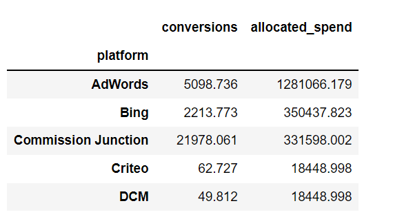
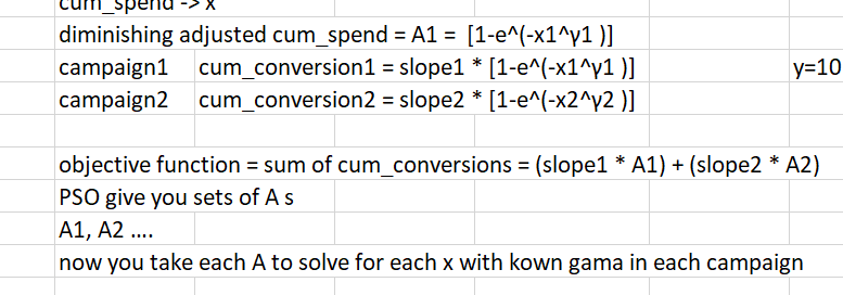
- After all the above processes are done, we calculate the conversions for every campaign by multiplying the spend coefficient with the allocated dollars, thus obtaining our cumulative conversion for that platform campaign. Then we aggregate the cumulative allocated dollars and cumulative conversions at the platform level and show the results. For the diminishing effect model, the optimization happens on diminishing adjusted cumulative dollars. So, the formula becomes (Coefficient * Diminishing effect adjusted cumulative dollars) and we solve for the Spend using the later for the optimum solution.